Saleae Logic2 Analog filtering technical details?

[BitBob]

I am trying to understand the technical limitations of Saleae Logic’s analog inputs. I am aware of the support articles:

The Digital and Analog Recording on the Same Channel Appear Different

“In addition to the hardware AA filter, there is a digital-analog filter that engages for sample rates lower than the advertised sample rate. This is called the decimation filter. It will filter the data further before down sampling so data sampled at lower rates does not suffer from aliasing from frequency components that made it through the analog AA filter.”

Device Settings Configuration Tips

“To accurately record an analog signal, you must sample at least 10 times faster than that signal. That is due to the filter response of our down-sampling filter as well as the hardware anti-aliasing filter that defines the maximum analog bandwidth of the device.”

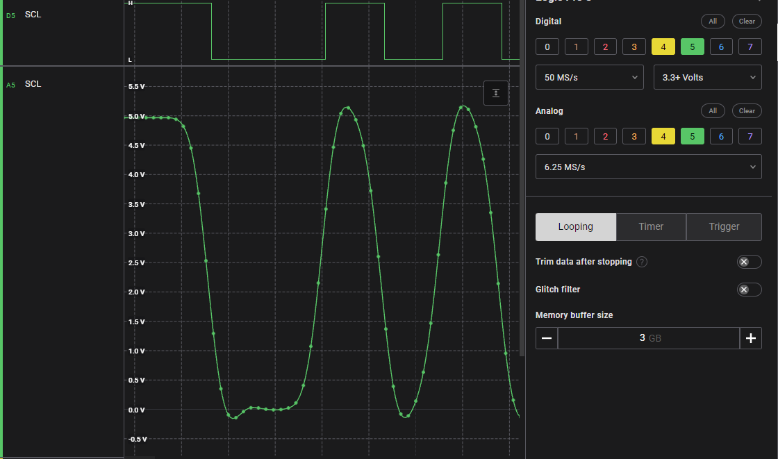
… however, I was surprised at the apparent ‘extra filtering’ (in a software guys opinion) coming through on what I thought were ‘sufficiently extra’ sample frequencies when studying I2C signals. See picture below – plotting the SCL analog voltage sampled at different frequencies (50 MS/s, 6.25 MS/s, and 3.125 MS/s) as well as the ‘digital’ signal (@500 MS/s).

Note: these are all for an I2C SCL frequency of 400 kHz

So, the questions are:

1. What are the electrical characteristics of the HARDWARE filter on analog channels? Per datasheet, claim 5 MHz bandwidth on 50 MS/s data, so I assume a low-pass RC filter? Can you share the R & C values / details on this?

2. What exactly is the software ‘decimation filter’ implemented when selecting other analog sample frequencies besides 50 MS/s? Also, is this filtering implemented within the FPGA (ahead of USB data stream) or on the PC side (after USB received to Logic2 software)?

3. Any chance we could (optionally) turn OFF the software ‘decimation filter’ and just do an ‘unfiltered decimation’ simple down sampling instead? Yeah, I know that Nyquist sampling theorists will scream about risks of aliasing – but you can only alias signal that actually exists on the input.

If we have our own hardware filtering (R’s and C’s), then we (hopefully) shouldn’t need any extra software filtering – and I’d like to have less ‘rounded’ and ‘attenuated’ analog waveform that is >10X my underlying operating frequency. Unfortunately, these digital clocks are not sinusoidal, they are square waves – so the software filtering can lose the sharp edges and signal peaks & valleys that I’d still like to see.

A quick follow-up:

I found a YouTube video that discusses more about the aliasing topic.
Per: https://youtu.be/UHwyHcvvem0&t=7m7s
… it seems like the minimum sample rate for 400 kHz SCL should be:
3 x 2.5 x 400 kHz == 3 MHz

However, neither the 3.125 MS/s nor the 6.25 MS/s settings appear to capture the ‘complex’ (square) waveform, but rather it seems to be filtered down to a more sinusoidal wave (as though I’m being bandwidth limited by the decimation filter built in to Saleae’s analog signal chain?)

Finally, here’s a clip discussing more about bandwidth limitations affecting the captured waveform: https://youtu.be/9AJRaDJ0ofQ&t=2m59s

In this example – just changing scope’s bandwidth setting from 1 MHz to 5 MHz seemed to ‘square up’ the 1 MHz square wave (5X bandwidth) better than I could capture on the Saleae Logic with a sample rate setting over 15X vs. fundamental frequency (i.e., the 6.25 MS/s vs. 400 kHz SCL frequency still looks way more sinusoidal than the YouTube example).

Note: I realize I’m mixing the bandwidth vs. sample rate settings and the two are different, but I’m providing an example of the waveform capture behavior that I’m hoping to achieve.

The higher level point I’m trying to make, is that I believe the underlying analog data I want captured is technically available inside the Saleae hardware, so I’m looking for an option to see it rather than it being ‘lost’ in the analog signal chain. Maybe the decimation filter is bandwidth limiting more than the minimum required to provide the maximum visibility of higher frequency content?

For reference – here are some screenshots from the original Saleae Logic captures:

50 MS/s - clean picture (but 125X the SCL frequency):

6.25 MS/s - sinusoidal (but >15X the SCL frequency):

3.125 MS/s - sinusoidal and attenuated (even though ~8X the SCL frequency):

[timreyes]

@BitBob Besides sampling at the maximum advertised sampling rate for your device, we unfortunately don’t have a way of turning off the decimation filter manually.

You bring up some great points, and thanks so much for sharing a plot of the analog samples over time. It does seem to become ‘rounded’ when sampling at our recommended minimum sampling rate value of 10x the frequency of the signal.

I’ll need to pull together some of our team members to get their thoughts on the points you brought up and we’ll get back to you on this.

[BitBob]

Hi @timreyes, FYI –

I did another few experiments with a signal generator, with a ‘square wave’ output set to 2.5V peak-to-peak and 1.25V Offset and created an Excel chart with the combined CSV data exported (and zoomed in) from two separate captures:
Trial #1 (T01):
Saleae Logic Pro @50 MS/s analog
PicoScope @ ~3MS/s

Trial #2 (T02):
Saleae Logic Pro @3.125 MS/s analog
PicoScope @ ~3MS/s

Notice that the PicoScope analog data is apparently NOT as filtered even using a lower sample rate (i.e., ~3 MS/s vs. 3.125 MS/s).

I also noticed that the PicoScope 6 software has some sampling options, such as:

• Sin(x)/x Interpolation (I had this turned OFF in “Tools > Preference > Sampling”)
• Bandwidth Limit set to “None” (could have set to “20 MHz”) on the channel

I wasn’t sure if Saleae Logic2 software (or the FPGA firmware) is doing one (or both) of these settings (interpolation and/or bandwidth limiting) automatically, and without user-configurable method to turn the feature(s) OFF?

E.g., had the software/firmware done a simple sample decimation, then I expect the results would have been pretty similar to the PicoScope – the waveform would have been more ‘square’ than ‘sinusoidal’ and would NOT have been attenuated either.

I look forward to better understanding the analog signal chain design – as I use my Saleae Logic Pro more for its digital features, but it would be nice to more fully exploit the analog capabilities, too (without unnecessarily wasting memory @50 MS/s).

[Edit: update]

I did some additional analysis with the waveform generator and the Saleae Logic2 software ‘Measurement’ tool, and found some data to indicate that the decimation filter frequency response may be below 400 kHz for the 3.125 MS/s analog sample rate?

E.g., given waveforms w/ 2.5Vpp and +1.25V offset:

[Correction] 1.25V * SQRT(2)/2 + 1.25V = ~2.13V (~3 dB point)
[was: 2.5V * SQRT(2)/2 = ~1.77V – but 2.5V isn’t the right signal magnitude]

Set analog capture to 3.125 MS/s sample rate

400 kHz Square:
Vpp 1.5977706909179688 V
Vmin 0.45788028836250305 V
Vmax 2.0556509494781494 V (~0.64 gain)
Vavg 1.2542787790298462 V
Q5% 0.47309714555740356 V
Q95% 2.0404341220855713 V

490 kHz Square:
Vpp 1.0296744108200073 V
Vmin 0.7419284582138062 V
Vmax 1.7716028690338135 V (~0.42 gain)
Vavg 1.2574741840362549 V
Q5% 0.7520729899406433 V
Q95% 1.7614582777023315 V

490 kHz Sine:
Vpp 0.8064938187599182 V
Vmin 0.8535187840461731 V
Vmax 1.6600126028060913 V (~0.33 gain)
Vavg 1.2538232803344727 V
Q5% 0.8585910797119141 V
Q95% 1.6508824586868285 V

444 kHz Sine:
Vpp 1.0347466468811035 V
Vmin 0.7368561625480652 V
Vmax 1.7716028690338135 V (~0.42 gain)
Vavg 1.2547069787979126 V
Q5% 0.7470007538795471 V
Q95% 1.7614582777023315 V

Am I missing something, or analyzing this wrong … ?

[Edit: - added +1 waveform measurements, and updated gain calculations above]

297 kHz Sine:
Vpp 1.7499394416809082 V
Vmin 0.3817959427833557 V
Vmax 2.131735324859619 V (~0.71 gain)
Vavg 1.2577297687530518 V
Q5% 0.3970127999782562 V
Q95% 2.1215908527374268 V

Finally, an external reference for more about ‘decimation’ and ‘downsampling’ :

Decimation - dspGuru

[timreyes]

@BitBob Thanks for all of the added info! I’ll add your additional notes to our backlog.

[markgarrison]

Hi @BitBob, nice workup!

I developed the digital filters used for our products.

First off, I did want to mention that back when we were developing these products, we spent quite a lot of time discussing exactly how we wanted to handle down sampling. When we first launched the products, we included a CIC filter in the FPGA to filter the data (and downsample it at the same time) to ensure that signal content between the new, lower Nyquist rate and the original Nyquist rate would be appropriately suppressed. Later, we removed that from the FPGA implementation completely, and the FPGA now performs a simple downsample.

However, the reason the data is filtered in the SW is actually caused by another Issue. The frequency response of the hardware filter was never designed to be flat - there is a discontinuity at a fairly low frequency (I think around 100 kHz) which is there to ensure that over the tolerance range of the capacitors of the filter, the filter would still keep the advertised signal voltage range inside of the ADC rails.

To correct for this, 100% of recorded analog data is run through a calibration filter which compensates for this, but also limits the bandwidth. I don’t recall now why exactly we standardized on 1/10th the sample rate as the bandwidth for each filter, but I suspect it had to do with filter stability. In order to filter the data fast enough (especially on 2014 era PCs) we needed to use a IIR filter with a low number of coefficients, in order to keep up in real time at the maximum rate, (5x50MS/s).

This calibration filter is unique to each device, channel, and downsample rate. This is 95% of the calibration file that is downloaded the first time you use the device. (The other 5% is DC calibration, a simple gain & offset coefficient that maps ADC codes to volts)

If you delete the calibration file from your machine, and then disconnect from the internet (or otherwise block Logic 2 from downloading the calibration file), you can still record data - although you will get a lot of warming messages about calibration missing. This will allow you to see the unfiltered data.

Also one last thing - I went looking to see exactly when we removed the CIC filter from the FPGA. I’m not actually sure now. We talked about doing it a pretty long time ago, but reading the commit history, I’m not sure it was ever removed for the Xilinx based version of the products. (during the 2021 supply chain issues, we switched to Lattice FGPAs)

The lattice variant of the device definitely does not have a CIC filter. However, unless I’m missing something, it looks like we didn’t actually delete it from the Xilinx design.

Details on how to check your HW revision here: Logic Hardware Revisions - Saleae Support

Revisions 4, 5, 6, 9, 10, and 11 are all Lattice based.

We have no plans to go back and make adjustments to the FPGA image at this point. I will say that for future products, we will be sure to not additionally filter when downsampling.

Your questions:

1. The hardware uses a Bessel filter:
   

   

2. The decimation filter, for Xilinx based devices, is a CIC filter. It’s been a really long time since I’ve thought about that, but I don’t think CIC filters have any parameters other than the downsample rate. They are very simple filters. For the newer HW revisions, there is no downsampling filter in the FPGA.

3. There is no easy way to do this. The recommendation for maximum bandwidth is to sample at the maximum sample rate, at the cost of the number of channels you can record and the very high memory consumption rate. You can try disabling the calibration as mentioned above, but that will leave you with poor frequency flatness, and non-trivial DC offset and gain error. That said, the calibration file format is quite simple, and you could try editing the filter parameters. For example if you wanted to keep the DC accuracy, but eliminate IIR filter completely, you could edit the taps lists to contain a single 1.0 for the first tap (feed forward) and replace the rest with 0.0s. However, you would still loose the frequency response flatness. It would be fairly non-trivial to try and re-compute that. If you’re interested, if you send me your device ID, I can retrieve the original factory calibration information, including the measured frequency response with no filtering.

[BitBob]

Hi Mark –

Thank you for your detailed response; I am definitely interested in tweaking my calibration settings, so I will send in a separate support ticket with my HW serial number details to get more details on my original factory calibration data. I do have an ‘original’ version (Rev. 0.0.0) that has the Xilinx FPGA, as per:

Logic Hardware Revisions

For other’s reference, I found the Saleae support article:

Device Calibration

… which provides more information about the device-specific calibration file.

Meanwhile, as far as decimation vs. down-sampling, I did subsequently find another article:
https://www.ni.com/docs/en-US/bundle/labview-digital-filter-design-toolkit-api-ref/page/lvdfdtconcepts/dfd_decimation.html

… that gives some good insight into why/how you should implement a decimation (anti-aliasing) filter when changing (reducing) sample rates, as well as links to a more general discussion about multi-rate filtering (rational resampling, interpolation and decimation).

From what I’ve gathered, it can be important to properly process your signal chain to prevent aliasing – and I understand that typically means doing a filter before down-sampling (decimation), as that is the best way to keep the signal ‘clean’ from any of the aliasing artifacts. Thus, I would think that some type of decimation filter would be expected on the device-side of the USB connection, assuming that a lower sample rate setting means that less data is actually sent over the bus (i.e., the FPGA is down-sampling vs. the PC host software).

Ultimately, I’d check with an expert in the digital signal processing domain, as I know that this subject is quite complicated to get it done ‘right’ (where the definition of ‘right’ needs to be optimized and tailored to your design constraints, including any performance constraints to support older PCs). All I know, is that the waveforms above seemed ‘wrong’ to me – but I’m learning a lot about why such side-effects may actually be necessary in order to preserve the integrity of a signal when capturing at various sample rates.

Thanks!

PS: Kudos to Saleae – it isn’t every company that is willing to provide such detailed technical design disclosures, nor elicit a response from a company co-founder on the public support forum . (May you never let your company be overrun by Ivy league bean-counters and lose sight of making great products)

Ultimately, I’m just trying to improve the performance of this awesome little box – as it is quite a game-changer for me vs. trying to do repeated tests to optimize my trigger & capture settings on a traditional oscilloscope in order to get a snapshot that actually both captures enough range & resolution, and still triggers at the right (or close enough) timeframe. Instead, my Saleae Logic 2 allows me to just hit the ‘start’ button once to save the seconds/minutes/hours-long capture and then analyze everything after-the-fact. With this capability, I rarely miss catching the important information (especially for digital data). I’m hoping for an enhancement to in the analog capture capability, as I’d prefer to not need to store minutes (or hours) of 50 MS/s analog data just to see 400 kHz square waves “accurately enough” .

[Edit]
Also, I found some background info on the calibration process from Saleae’s blog back in 2014:

Logic 8 Update – the Home Stretch

[BitBob]

A follow-up question specific to the comment about editing the device-specific calibration file.

I was able to download my device’s *.cal file (per links in prior reply), and see the following XML tags for the mCalibrationData tag:

		<mCalibrationData class_id="3" tracking_level="0" version="0">
			<count>96</count>
			<item_version>16</item_version>
			<item class_id="4" tracking_level="0" version="16">
				<mChannel class_id="5" tracking_level="0" version="16">
					<mDeviceId>XX(my-device-id in decimal)XX</mDeviceId>
					<mChannelIndex>0</mChannelIndex>
					<mDataType>0</mDataType>
				</mChannel>
				<mSampleRate>50000000</mSampleRate>
				<mDf1SosCoefficients>
					<count>30</count>
					<item_version>0</item_version>
					<item>1.08689917156175</item>
						:  // (total of 30 <item> tags)
				</mDf1SosCoefficients>
				<mFirTaps>
					<count>30</count>
					<item_version>0</item_version>
					<item>1.08689917156175</item>
						:  // (total of 30 <item> tags, seem to all match mDf1SosCoefficients above)
				</mFirTaps>
				<mGroupDelay>3</mGroupDelay>
				<mImpulseLength>2993</mImpulseLength>
			</item>

			:  // (total of 96 <item> tags, one for each mSampleRate(6 rates) x mChannelIndex(16 channels))

Note: on my Saleae Logic Pro 16, this repeated for a total of 96 entries, one for each:

• mSampleRate (6 total) = {50M, 12.5M, 6.25M, 3.125M, 1.5625M, 781.25k}, AND
• mChannelIndex (16 total) = [0…15]

So, to properly ‘eliminate the IIR filter completely’ – should I change the above sections (all 96 entries) as follows (e.g., for 50MS/s mSampleRate entry):

				<mSampleRate>50000000</mSampleRate>
				<mDf1SosCoefficients>
					<count>30</count>
					<item_version>0</item_version>
					<item>1</item>
					<item>0</item>
					<item>0</item>
					<item>0</item>
					<item>0</item>
					<item>0</item>
					<item>0</item>
					<item>0</item>
					<item>0</item>
					<item>0</item>
					<item>0</item>
					<item>0</item>
					<item>0</item>
					<item>0</item>
					<item>0</item>
					<item>0</item>
					<item>0</item>
					<item>0</item>
					<item>0</item>
					<item>0</item>
					<item>0</item>
					<item>0</item>
					<item>0</item>
					<item>0</item>
					<item>0</item>
					<item>0</item>
					<item>0</item>
					<item>0</item>
					<item>0</item>
					<item>0</item>
				</mDf1SosCoefficients>
				<mFirTaps>
					<count>30</count>
					<item_version>0</item_version>
					<item>1</item>
					<item>0</item>
					<item>0</item>
					<item>0</item>
					<item>0</item>
					<item>0</item>
					<item>0</item>
					<item>0</item>
					<item>0</item>
					<item>0</item>
					<item>0</item>
					<item>0</item>
					<item>0</item>
					<item>0</item>
					<item>0</item>
					<item>0</item>
					<item>0</item>
					<item>0</item>
					<item>0</item>
					<item>0</item>
					<item>0</item>
					<item>0</item>
					<item>0</item>
					<item>0</item>
					<item>0</item>
					<item>0</item>
					<item>0</item>
					<item>0</item>
					<item>0</item>
					<item>0</item>
				</mFirTaps>

What about the mGroupDelay or mImpulseLength tags? Is the Logic 2 software also ‘time-shifting’ the analog signal based on these parameters (i.e., to try and correct for any group delay of the IIR filter)? If so, should these values be modified as well?

Thank you!

[BitBob]

Hey @markgarrison –

I tried the above modifications to the calibration file, and then manually loaded it in, by:

1. Removing the original calibration file from %APPDATA%\Logic\calibrations\
2. Disconnecting computer from network (airplane mode / disabled Ethernet connection)
3. Manually “Load” the modified *.cal (just channel 0 for now)
4. Confirmed a new calibration file appeared in %APPDATA%\Logic\calibrations\
5. Renamed the new calibration file to exactly match original filename

Screenshot of “Device Calibration Error” dialog (used to manually load):

Note: In the first trial, the filename was different than the original, in the pattern:
[device-id-in-decimal]-[other-number]-1.cal

… where the [other-number] didn’t match the original. When I reconnected network, it appears that the Logic software auto-downloaded the original calibration and that took effect (making the CH0 / CH1 behavior appear to match).

So, the second time, I added step #5 (rename JSON *.cal file to match original filename), and it looks like Logic didn’t try to auto-download the original this time.

However, by making the modifications outlined in previous post (first is 1, the other 29 are 0), the signal was completely flatlined for CH0:

I looked inside the calibration file created from step #3/4 above, in %APPDATA%\Logic\calibrations\ and found (embedded for the 50MS/s setting):

{"groupDelay":3,"impulseLength":2993,
 "df1SosCoefficients":
 [{"b0":1,"b1":0,"b2":0,"a1":0,"a2":0},
  {"b0":0,"b1":0,"b2":0,"a1":0,"a2":0},
  {"b0":0,"b1":0,"b2":0,"a1":0,"a2":0},
  {"b0":0,"b1":0,"b2":0,"a1":0,"a2":0},
  {"b0":0,"b1":0,"b2":0,"a1":0,"a2":0}]}

As you can see, the translation of list (30 items) in the XML formatted calibration file appears to be translated into to 25 (??) values in the JSON formatted file.

Thus, I am guessing that a different pattern of values needs to be used vs. just setting first to 1 and the other 29 to 0.

The mapping from XML to JSON appears to be as follows:

					<item>b0</item>
					<item>b1</item>
					<item>b2</item>
					<item>"1"</item>
					<item>a1</item>
					<item>a2</item>

Where the 4th line is always a constant “1” and didn’t appear to translate from XML to JSON file, which likely explains the discrepancy of 25 vs. 30 item entries above (it is the understood a0 = 1 term in the denominator?)

Here’s what I believe to be the full mapping:

					<item>b0[0]</item>
					<item>b1[0]</item>
					<item>b2[0]</item>
					<item>"1"[0]</item>
					<item>a1[0]</item>
					<item>a2[0]</item>
					<item>b0[1]</item>
					<item>b1[1]</item>
					<item>b2[1]</item>
					<item>"1"[1]</item>
					<item>a1[1]</item>
					<item>a2[1]</item>
					<item>b0[2]</item>
					<item>b1[2]</item>
					<item>b2[2]</item>
					<item>"1"[2]</item>
					<item>a1[2]</item>
					<item>a2[2]</item>
					<item>b0[3]</item>
					<item>b1[3]</item>
					<item>b2[3]</item>
					<item>"1"[3]</item>
					<item>a1[3]</item>
					<item>a2[3]</item>
					<item>b0[4]</item>
					<item>b1[4]</item>
					<item>b2[4]</item>
					<item>"1"[4]</item>
					<item>a1[4]</item>
					<item>a2[4]</item>

So, is the internal filter implementation using 5 cascaded second order IIR filters?

Thus, assuming the IIR filter equation is:
y(n) = b0 * x(n) + b1 * x(n-1) + b2 * x(n-2) - a1 * y(n-1) - a2 * y(n-2)

… I think I’d want to set b0 = 1, and set b1 = b2 = a1 = a2 = 0 (in order to get y(n) = 1 * x(n))?

Therefore, I think the right list should be as follows:

					<item>1</item> // b0[0]
					<item>0</item> // b1[0]
					<item>0</item> // b2[0]
					<item>1</item> // a0[0] = 1
					<item>0</item> // a1[0]
					<item>0</item> // a2[0]
					<item>1</item> // b0[1]
					<item>0</item> // b1[1]
					<item>0</item> // b2[1]
					<item>1</item> // a0[1] = 1
					<item>0</item> // a1[1]
					<item>0</item> // a2[1]
					<item>1</item> // b0[2]
					<item>0</item> // b1[2]
					<item>0</item> // b2[2]
					<item>1</item> // a0[2] = 1
					<item>0</item> // a1[2]
					<item>0</item> // a2[2]
					<item>1</item> // b0[3]
					<item>0</item> // b1[3]
					<item>0</item> // b2[3]
					<item>1</item> // a0[3] = 1
					<item>0</item> // a1[3]
					<item>0</item> // a2[3]
					<item>1</item> // b0[4]
					<item>0</item> // b1[4]
					<item>0</item> // b2[4]
					<item>1</item> // a0[4] = 1
					<item>0</item> // a1[4]
					<item>0</item> // a2[4]

And, it looks like this updated method is achieving closer the desired results:
For all waveforms below, CH0 is the “modified” calibration file (per above), while CH1 is using “factory original” values for that channel.

Capture at 50 MS/s:

Capture at 12.5 MS/s:

Capture at 6.25 MS/s:

Capture at 3.125 MS/s:

(Note: the curviness & camel hump appearance is likely due to display graphics connecting the dots – using a curve fit vs. straight lines?)

So, I’m now curious about exactly how the IIR filter is being applied?
Is the IIR filtering being applied AFTER the down-sampling (and CIC decimation filter?) that is done in the FPGA firmware? I would expect that down-sampling is done on the FPGA side to reduce the USB data congestion for higher channel counts, right?

Thus, is the input/output of these IIR filters all run AFTER the data was down-sampled (in the FPGA?), at the analog sample rate set in the GUI?
OR - is the analog down-sampling (and some level of anti-aliasing filtering) still being done on the PC/host side, such that the FPGA sends analog data over USB at some higher sample rate vs. the GUI setting, and the sample rate setting reduces the PC storage demands, but not necessarily the USB overhead?

Finally, how does this analog signal chain differ between FPGA firmware / hardware revisions?
(e.g., I understood from your previous reply that v0.0.0 w/ Xilinx FPGA still has CIC decimation filter done on the FPGA side before USB data is streamed to the PC and possibly down-sampled for settings < 50 MS/s)

Thanks again for helping me ‘deep-dive’ to understand the analog behavior & performance of the Saleae Logic

[Edit: I forgot to mention – it looks like I needed to zero out the mGroupDelay setting vs. calibrated value, or else the ‘modified’ analog data was coming earlier than the ‘factory’ data (which seems to indicate that the GUI is time-shifting the filtered analog data based on the group delay … ?) If so, is there any side-effect to the mImpulseLength value, as I left those in the original factory calibration setting for now?]

Capture @50 MS/s with original factory calibration setting of mGroupDelay = 3:

(it looks like the A0/CH0-Mod data was time-shifted by ~3 sample points earlier than other waveform (??))

Zoom in of previous capture @50 MS/s with modified mGroupDelay = 0:

[markgarrison]

Hi @BitBob,

I’m glad you’re interested! I’ve emailed you a copy of your device’s factory test data. You can try plotting that on a log/log graph to see that frequency response effect I was talking about, which is why we include a calibration filter in the calibration file.

After reviewing your posts, I think I can cover all of your questions with the following background information.

Why we don’t plan to add down sampling AA filters again for future analog products.

To clarify, future analog inputs will still have AA filters, but these will be fixed, and will be tuned for the bandwidth of the device. Anti-aliasing filters are quite important for many signal recording applications, especially those where frequency content is quite important. However, something we’ve learned after launching these products is that for oscilloscopes, and many other time domain signal analysis areas, aliasing can actually be a good thing. anti-aliasing filters can hide real signal components, filtering out quite a lot of information. In time domain, when a signal is heavily aliased, it shows up as an unmissable pattern which should quickly inform the user that there is higher frequency content in the signal they can’t see properly. At least in the scopes we tested, they made no attempt to filter the data before down sampling (when zoomed out in time), and for the use cases we’ve looked at, seeing the aliased signal was greatly preferable compared to seeing a nicely filtered signal that would indicate that no higher frequency content is present. I don’t know if all scopes lack AA down sampling filters, or just the ones we tested. (Note, I did these evaluations a very long time ago, and I don’t remember the specifics)

XML vs. JSON calibration files

The XML file is the original, official calibration file format, which we still generate at the factory for new units. This is the native format used by the Logic 1 software.

For Logic 2, we internally convert it to a more structured format. The Logic 2 software converts the XML file to the JSON format.

Every time the software detects a device is connected, it will check to see if a new calibration file is available, even if it has already downloaded a calibration file. Our calibration server provides the last updated date of each calibration file, and the software checks that against the local file. If the local file is older than the date returned by the server, the software will download the new file, over-writing the original. In practice, the only time we updated calibration files were released was shortly after we started shipping, when we needed to release DC calibration without AC support, as mentioned in that blog post you found.

The filename format you mentioned is as follows:
${deviceId}-${lastUpdated}-${PARSING_VERSION}.cal
The -1 at the end of the filename is there in case we need to change the JSON format, which would require all existing json files to be ignored and regenerated.

If you modify the json calibration file and restart the software, your modifications should be loaded into the application.

If you delete the json file, then a new XML file will be downloaded (ignoring any existing file), then it will be converted to json and saved.

Your analysis of the filter is correct, and yes changing b0 to 1.0 and the rest to 0.0 should result in a identity filter.

There is one filter definition for every sample rate of every channel. Note that really low samples rates, 625 KS/s and lower, actually only decimate to ~3 MHz in the hardware. We run the calibration filter at this data rate, then perform additional decimation in the software down to the final rate.

Where the filter is run

In your Xilinx based unit, there are 2 filters in the signal chain.

First is the CIC filter in the FPGA. this combines filtering and down sampling into one operation. Like you mentioned, we down sample in the FPGA to reduce USB bandwidth needs. This allows you to record more signals at once, record digital signals faster, and uses less bandwidth which generally makes the USB stream more reliable for long duration captures. CIC filters do not have any taps, instead we just specify the down sample ratio. That data is streamed to the PC, where we use the PC CPU to run the calibration filter on the data stream. This implementation is heavily optimized, and will automatically use SSE2, AVX, or AVX2 CPU instructions depending on what CPU you have.

Group Delay

It’s been a really long time since I’ve had to work on this, but one tricky part of building a mixed signal device (analog and digital recording) is getting the digital and analog signals properly synchronized. There is considerably different delays between the voltage at the input pin and when the data is captured by the FPGA, and then further delays are inserted by the various filters.

In short, we have a basic fixed model for the delay from the fixed components. in the analog path, relative to the digital path, the main contributing factors are the AFE group delay (including the analog filter), the ADC pipeline latency, and the latency between the ADC and the FPGA. The CIC filter adds it’s own delay, which is fixed, and then the calibration filter adds more delay, which varies filter to filter, which is why it’s stored in the calibration file.
Also stored in the calibration file is the filter impulse response. This is important because this is effectively how long the filter takes to “warm up”. If you simply start up an IIR filter, using zeros for the input and output history you don’t have, you will often get garbage data up until the impulse response length. Our software will discard these “warm up” output samples, to make sure that the first data you see is correct.
Note that the group delay and the impulse response length work to partially cancel each other out, as the way to compensate for delays in the signal path is discard samples from the start.

Interpolated lines in the UI.

When you zoom into the signal to the point where the data points are more than 1 horizontal pixel apart, we will draw smooth lines connecting the points. We use cubic spline interpolation for this. Fun fact, we tried several more traditional up sampling filters, and none were as a good at actually connecting the points.

Lastly, to see why the calibration filter is really needed, I recommend recording a 1KHz square wave. Zoom out to look at the whole wave, with and without filtering. I recommend taking a look at this at 50 MS/s, but lower rates should still capture the effect. I can see the effect in some of the screenshots you have shared, but it’s much more pronounced at lower frequencies.

[BitBob]

Hi @markgarrison –

Thank you for the detailed feedback and additional information. It may take a while to fully digest all of the details, but I am definitely getting a much better understanding of what is going on. Just to clarify a few items, the CIC filter you mention is just implementing:
https://en.wikipedia.org/wiki/Cascaded_integrator�%8 0%93comb_filter

… specifically:

(copied image from Wikipedia article above)

Where:

• R = {4,8,16,32,64} (for [12.5 … 0.78125] MS/s down-sample rates from 50 MS/s ADC input)
• M = 1 (number of samples per stage)

Meanwhile, I did see some of the possible analog artifacts in the 1 kHz waveform capture when the filtering is removed (as before, “CH0-Mod” has the modified calibration w/ ‘unity’ filtering coefficients, vs “CH1-Factory” is original factory calibrated filters):

And, viewing same waveform as an Excel X-Y scatter chart:

… zooming into the rising edge peak/transition:

(unfiltered channel is more rounded toward 2.5V vs. a more ‘square’ edge on the filtered channel – thus the ‘unfiltered’ result is off by ~0.2V … ?)

… extra zoom to show ‘ringing’ on the edge:

(as the ‘real’ signal is supposed to be [0 - 2.5] V range square wave, this plot makes it clear that the ‘unfiltered’ channel is not returning/stabilizing at 2.5V as quickly as the channel w/ filtering applied)

So, I see that removing the software filter completely can have a different trade-off than keeping the filter in place; maybe the real question now, is whether a ‘better’ filter could be implemented with the existing framework that improves the high-frequency performance (i.e., keeps the square waves square like previous response) without having as much of the lower frequency ‘rounding’ on edges as seen in the screenshots above when no filtering is applied.

To even attempt that – can you confirm if this is the software IIR filtering signal chain:
given x(n) is the 'n’th sample from USB receive buffer, then (in simplified terms):

• y[0] = IIR(x(n), coef[0])
• y[1] = IIR(y[0], coef[1])
• y[2] = IIR(y[1], coef[2])
• y[3] = IIR(y[2], coef[3])
• y[4] = IIR(y[3], coef[4]) = final output to capture/display

Note: coef[i] is the 'i’th set of IIR filter coefficients described previously: {b0[i] … a2[i]}

… or more specifically:

• y0 = b0[0] * x(n) + b1[0] * x(n-1) + b2[0] * x(n-2) - a1[0] * y0 - a2[0] * y0
• y1 = b0[1] * y0 + b1[1] * y0 + b2[1] * y0 - a1[1] * y1 - a2[1] * y1
• y2 = b0[2] * y1 + b1[2] * y1 + b2[2] * y1 - a1[2] * y2 - a2[2] * y2
• y3 = b0[3] * y2 + b1[3] * y2 + b2[3] * y2 - a1[3] * y3 - a2[3] * y3
• y4 = b0[4] * y3 + b1[4] * y3 + b2[4] * y3 - a1[4] * y4 - a2[4] * y4

(i.e., it is a cascaded IIR filter, as per the coefficients described in previous reply – where the first coefficient entries are applied first to the ‘raw’ ADC data from USB receive buffer and the later coefficient entries are applied last in the filtering chain?)

Thank you once again for the excellent feedback – and I’m still hoping that this discussion could result in a significant improvement in the analog capture performance characteristics by tweaking the software filtering methodology. It is good to know that this ‘problem’ isn’t buried deep within the FPGA firmware, but rather a ‘simple’ tweak to a calibration file (for someone who knows how to re-design the digital filtering coefficients).

[BitBob]

Assuming that the equations above were right, I tried to manually use the coefficients from the *.cal file into Excel, and got the following result (new grey line for IIR:y_4 added):

And, this seems right, given that I didn’t try to time-shift anything based on the mGroupDelay as discussed previously (and it appears that the data is off by about 3 points, consistent w/ mGroupDelay = 3 in the calibration file).

So, it seems like everything is all ‘adding up’ – just not sure about the best way to actually re-design a filter to improve the bandwidth, yet.

Thanks again!

[Sebastian]

Hi folks, I’m following this discussion with interest. I have a hard time to understand all the filtering details. But I also experience quite some frustration when my Logic Pro 16, or the PC software, puts the analog measurements at lower that 50Ms/s artificially onto some sine wave, often spoiling the analog analysis of digital signals with their steep edges. See for instance a 1MHz square wave sampled at 12.5Ms/s:

So if there is any way to massage the calibration file to disable or at least reduce some of this “sinusoidal smearing”, please help!

KR, Sebastian

[BitBob]

Hi @Sebastian –

As mentioned above, you can get your device-specific calibration file from Saleae’s download site, as per the reference linked in the thread above.

Within that file, you can modify the filter coefficients as described later in the thread above, namely:

1. Changing filter coefficients (mDf1SosCoefficients and mFirTaps) to b0 = 1, and set b1 = b2 = a1 = a2 = 0 (both sections)
2. Changing mGroupDelay value to 0

For example, here’s some snippets within the *.cal file to be modified:

				<mDf1SosCoefficients>
					<count>30</count>
					<item_version>0</item_version>
					<item>1</item> <!-- b0[0]     -->
					<item>0</item> <!-- b1[0]     -->
					<item>0</item> <!-- b2[0]     -->
					<item>1</item> <!-- a0[0] = 1 -->
					<item>0</item> <!-- a1[0]     -->
					<item>0</item> <!-- a2[0]     -->
						:
					<item>1</item> <!-- b0[4]     -->
					<item>0</item> <!-- b1[4]     -->
					<item>0</item> <!-- b2[4]     -->
					<item>1</item> <!-- a0[4] = 1 -->
					<item>0</item> <!-- a1[4]     -->
					<item>0</item> <!-- a2[4]     -->
				</mDf1SosCoefficients>
				<mFirTaps>
					<count>30</count>
					<item_version>0</item_version>
					<item>1</item> <!-- b0[0]     -->
						: <!-- exact same <item> list as above -->
				</mFirTaps>
				<mGroupDelay>0</mGroupDelay>

… modify the same way for all the (desired) sample rates:

				<mSampleRate>50000000</mSampleRate>
				<mSampleRate>12500000</mSampleRate>
				<mSampleRate>6250000</mSampleRate>
				<mSampleRate>3125000</mSampleRate>
				<mSampleRate>1562500</mSampleRate>
				<mSampleRate>781250</mSampleRate>

… and across all (desired) channel indexes:

				<mChannelIndex>0</mChannelIndex>
				<mChannelIndex>1</mChannelIndex>
				<mChannelIndex>2</mChannelIndex>
				<mChannelIndex>3</mChannelIndex>
						:
				<mChannelIndex>7 (or 15)</mChannelIndex>

And once you’ve modified the *.cal file, you need to load it into the Saleae Logic 2 software by:

1. Removing the original calibration file from %APPDATA%\Logic\calibrations\
2. Disconnecting computer from network (airplane mode / disabled Ethernet connection)
3. Manually “Load” the modified *.cal (just channel 0 for now)
4. Confirmed a new calibration file appeared in %APPDATA%\Logic\calibrations\
5. Renamed the new calibration file to exactly match original filename

(see original follow-up above for more details on this process)

Note: you may want to apply the filter coefficient changes outlined above to only ONE channel (e.g., channel 0 only), so you can compare the behavior between ‘factory calibrated’ vs. ‘modified/unfiltered’ channel options. Also, I recommend backing up the original factory calibration file first, so you can revert everything back to ‘factory original’ condition as needed.

Upon making the above calibration changes – you should see less “sinusoidal smearing” (as you put it), but there could be other side-effects as indicated in my follow up response. In particular, the unfiltered behavior may have some signal attenuation and/or frequency response issues that aren’t present when using the factory calibrated setup (which is why the filtering is there in the first place).

Thus, I believe the only ‘off-the-shelf’ way to get the maximum responsiveness in the analog channels is to just use the maximum sampling frequency available. Otherwise, I think the filter coefficients would need to be redesigned for better high-frequency capture performance without the undesired behavior you get if the filters are completely removed. However, I’m not sure if that is technically possible, or not. Likewise, I think the ‘recalibration’ method might need to be customized per each device – so it is probably an activity that Saleae would need to handle on their side, if they wanted to provide this ‘enhanced higher-frequency analog’ capability at lower sample rates.

So, I submitted this thread as an ‘Idea’ over on the Ideas and Feature Requests forum:

Improve High-Frequency Analog Performance at Lower Sample Frequencies - Logic...

(so, feel free to up-vote for this feature so Saleae can know how many others want this capability, too )

[Sebastian]

Ok, I massaged the JSON calibration file as suggested to have my channels 12-15 unfiltered. The waveforms look much more square now, for sure!

But I also observe some other effects. Obviously the analog waveform is now slightly too early versus the digital channels. I guess this could be recompensated.

But there are other measurement artifacts becoming visible as well. For instance, when an 1MHz square wave sets in after some constant 4.87V period, at 50Ms/s the calibrated/filtered channels show min/max Voltages properly from 0.00V to 4.87V, whereas the channels with the filters removed as described above toggle (after the over/undershoots) between 0.19V and 4.68V only.

Also, it takes about 15us to set in to a new common mode voltage. In the above example, the voltage span changes from initially 0.38V and 4.85V within the course of those 15us to the final 0.19V/4.68V, and similar at 12.5Ms/s, 6.25Ms/s and lower sampling frequencies:

This effect becomes very prominent, in case of my device, at a square wave frequency of 31250Hz, at any sampling rate, which gets quite significantly distorted by this effect on the unfiltered channels:

So, those simplified settings are no silver bullet either, and I clearly marked my device that channels 12-15 are now unfiltered …

Kind regards, Sebastian

[BitBob]

Re: Obviously the analog waveform is now slightly too early versus the digital channels. I guess this could be recompensated.

This behavior is controlled by the mGroupDelay setting:

   <mGroupDelay>0</mGroupDelay>

Completely removed it for (unfiltered) channels. Note that the digital waveform is based on the analog voltage crossing a threshold – so it is expected that the analog waveform would be slightly ahead of the digital waveform. Thus, if the mGroupDelay was ‘perfectly timed’ then a marker placed at the digital edge would line up on the analog waveform at the digital logic threshold:

• 0.6V (for 1.2V logic setting)
• 0.9V (for 1.8V logic setting)
• 1.65V (for 3.3V logic setting)
  Or (for non-Pro models):
• 0.6V (low / falling edge) or 1.2V (high / rising edge)

Re: there are other measurement artifacts becoming visible as well
Yes, I found the same effects on the completely unfiltered output. I think some of the software filtering is attempting to ‘correct’ for the ‘raw’ analog data (i.e., countering some of hardware filtering artifacts?)

Meanwhile, I did play around a bit more with the filtering, and it appears that the staging is split into two parts (??), the y[0] filter appears to do the majority of the work countering the major artifacts of the ‘unfiltered’ signal, while the y[1] to y[4] are doing TBD additional filtering updates (but these stages appear to have the more significant cut-off frequency effects, too).

So, my modified recommendation is to keep the first 6 (of 30) entries in each filter with the original factory settings, and then replace the remaining 24 (of 30) entries to the ‘unity’ coefficients described earlier.

Specifically:

					<count>30</count>
					<item_version>0</item_version>
					<item>X</item> <!-- b0[0] = original value 'X' -->
					<item>Y</item> <!-- b1[0] = original value 'Y' -->
					<item>Z</item> <!-- b2[0] = original value 'Z' -->
					<item>1</item> <!-- a0[0] = 1 (original value) -->
					<item>P</item> <!-- a1[0] = original value 'P' -->
					<item>Q</item> <!-- a2[0] = original value 'Q' -->
						:
					<item>1</item> <!-- b0[1..4]     -->
					<item>0</item> <!-- b1[1..4]     -->
					<item>0</item> <!-- b2[1..4]     -->
					<item>1</item> <!-- a0[1..4] = 1 -->
					<item>0</item> <!-- a1[1..4]     -->
					<item>0</item> <!-- a2[1..4]     -->

Note: This seemed to improve the artifacts described above (better than ‘raw’ / completely unfiltered response) – but I’m not exactly sure what the remaining filter coefficients are accomplishing (@markgarrison ??)

Ultimately, I think it is up to Saleae (or somebody else who has a better DSP / IIR filter design background) to chime in and give a better answer. However, I did want to share my findings in case it helps anyone else looking for an improved high-frequency responsiveness (with TBD side effects vs. the ‘factory’ settings).

[Edit] – for those curious, here’s an updated chart where I added the y[0] (yellow) and y[4] (grey) filter outputs (calculated in Excel using the coefficients from the *.cal file) vs. the original factory calibration (on CH1 - orange) and the ‘Raw’ (unfiltered) output on CH0 (blue):

… zooming in a bit:

… and zooming in even more:

[Sebastian]

@BitBob

So, my modified recommendation is to keep the first 6 (of 30) entries in each filter with the original factory settings, and then replace the remaining 24 (of 30) entries to the ‘unity’ coefficients described earlier.

I’ll give that a try …

Kind regards, Sebastian

[Sebastian]

@BitBob, I wrote a little python script to massage the JSON calibration file as by your suggestion, see here:
massagecal-anonymised.py (688 Bytes).

Indeed those filter settings seem to achieve the goal without obvious negative side effects.

Digging deeper into the settings, I see that the higher order filter coefficients (coef[2], coef[3] and coef[4]) all have b1 set to 2 and b2 set to 1. Isn’t that dubious in the first place?

Btw, I found that in my case a groupDelay of -1 would be more appropriate for the simplified filter channel at all sampling rates (although for 781250 and 1562500, groupDelay of 0 and -1 were a tie).

[BitBob]

Hi @Sebastian –

Thanks for the Python script – it is quite handy for tweaking a *.cal (JSON format) file directly in the %APPDATA% (or equivalent) folder directly, rather than modifying the XML file and going offline to reload it. As far as understanding the other filter coefficients – I defer to @markgarrison as he is the best to give feedback on the overall analog channel filtering strategy, and what each stage was designed to do.

At this point, I think it would be nice (if Saleae agrees) to have a GUI setting/option for each analog channel to do what this script is essentially doing – similar to how other oscilloscopes can (optionally) ‘bandwidth limit’ a given channel. It could be toggled on a ‘per channel’ basis, and ON by default to preserve existing behavior.

For a given analog channel:

• When ‘bandwidth limit’ is ON:
  df1SosCoefficients = {factory default: all stages}
• When ‘bandwidth limit’ is OFF:
  df1SosCoefficients = { {factory default: first stage}, {b0=1; b1=b2=a1=a2=0: all other stages} }

Also, it would be nice to make it visible & accessible. However, depending on how ‘official’ of a setting this is considered by Saleae, I’d be content to just have it available – even if it is buried within an ‘expert mode’ field somewhere

Perhaps just duplicate the analog channel on/off method for a new Analog Bandwidth Limited setting? Something like:

[BitBob]

FYI –

Just an update on this topic. I did find some information about de-embedding filters on the EDN website that discusses the technical issues related to oscilloscope signals and having to compensate for the frequency-dependent variations in the signal due to various analog effects in the signal chain.

Thus, I am hypothesizing that the first IIR filter was providing the unit-specific de-embedding filter (to compensate for the high-frequency losses in the hardware), while the remaining IIR filters were providing some additional filtering that will ultimately limit the bandwidth of the analog channels when using lower analog sample rates. (@markgarrison – any comments?)

So, the python script provided above (by @Sebastian) can be used & tweaked to ‘zero-out’ the low-pass filters, while keeping just the factory calibrated de-embedding filter to avoid the side-effects described earlier.

Note: you will need to at least modify the script to point to your specific calibration file(s) and make some additional tweaks if you’re using a Logic with <16 channels or want to change which channels are being ‘bandwidth unlimited’ vs. using original factory calibration settings (as the original script above is hardcoded to ‘unfilter’ channels 12-15).